Generate Mobile Mapping Scans
The Generate Scans feature is to extract mobile mapping scans from the raw data files of the MX series mobile mapping systems (excluding the MX7). For the MX9 and MX90 raw data files, the process is done in two steps, from converting first the RXP laser format files to the TMX format files and then the TMX format files to the RWCX point cloud format files readable in TBC. For the MX50 and MX60 raw data files, the process is done in one step, from converting the TMX format files to the RWCX point cloud format files.
TMX files contain scan raw data with polar scan coordinates and intensity and timestamp information. RWCX files are point cloud format files, with intensity, color and normal information.
To generate mobile mapping scans:
- In the Project Explorer, right-click the Mission node (or any node under the Mission node) and select Generate Scans in the context menu.
- The Generate Mobile Mapping Scans dialog displays, with the mission selected by default, as well as all of the runs.
MX9 and MX90 - The pane below lists the devices (cameras and lasers) and the raw data files (MXIPS video format files, PGR video format files, and RXP laser format files) that are associated with a run when the run is selected.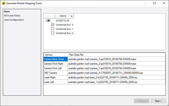
MX50 - The pane below lists the devices (camera and lasers) and the raw data files (TMX laser format files) that are associated with a run when the run is selected.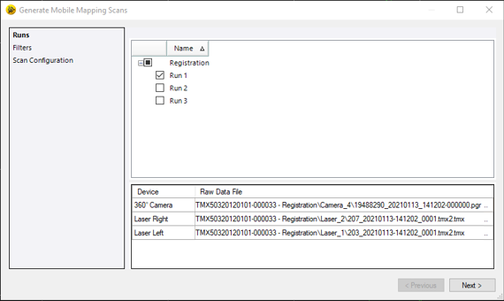
MX60 - The pane below lists the devices (cameras and lasers) and the raw data files (TMX laser format files) that are associated with a run when the run is selected.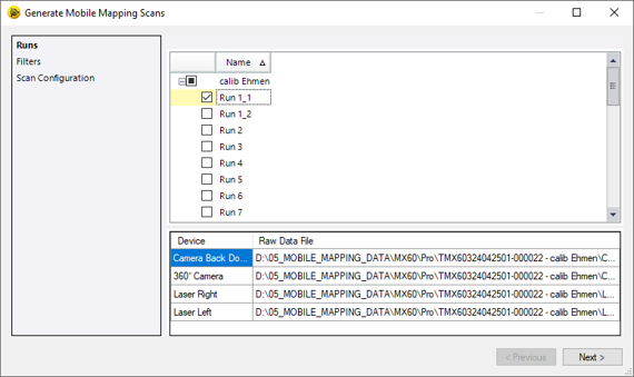
Note: In case there are several missions available into your project, you can only select and process runs belonging to the same mission.
From here, there are two (or three) steps to follow. The first step is to select one run (or more) to process, or all of them, i.e. the mission.
- Check the Mission option. All Runs are checked accordingly.
- Or check a Run option, and click Next.
MX9 and MX90 - Perform the steps below: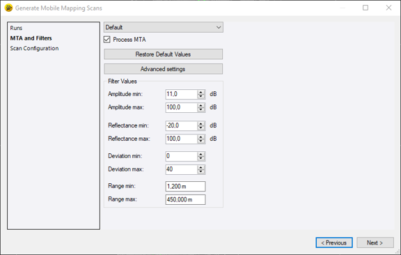
You can choose a filtering configuration among the three available (Default, Rail and Power Lines) to apply to the mobile mapping scans to extract. A filtering configuration contains a set of preset values for the following parameters: Amplitude, Reflectance, Deviation and Range.
When a laser scanner emits a laser pulse and it receives in return an echo signal. The Amplitude and Reflectance are the parameters of the echo signal, respectively the raw amplitude of the return pulse reaching the laser scanner and the surface (or target) reflecting property. The Amplitude is defined as the ratio of the actual detected optical amplitude of the echo signal versus the detection threshold of the scanner. Its value a ratio in the units of decibel (dB). Amplitude depends on the distance. Further away the scanner is from the target the less power it receives. The value of the Reflectance is a ratio in the units of decibel (dB). The Reflectance provided is a ratio of the actual optical amplitude of the target to the amplitude of a diffuse white flat target at the same range-reading. Its value a ratio in the units of decibel (dB). Negative and positive values of the Reflectance are directly dependent on the reflectivity of the surface (or target), diffusely reflecting for negative values and retro-reflecting for positive values. The difference between the Deviation Min. and the Deviation Max. is called Deviation Gate which refers to a filter allowing to filter mixed pixels (noise echoes between two objects of the same laser pulse). This filter can be used to delete pixels between rail-heads and the ground. Lower the Deviation Max. value will delete more mixed pixels. The Range Min. and Range Max. parameters refer to the minimum range and the maximum range the laser scanner is capable of performing range measurements. The difference between the maximum range and the minimum range is called Range Gate.
Default filter contains a set of presets inside which the Amplitude filtering is Off (values from 0 to +100) and the MTA processing is On (Auto mode).
Rail filter contains a set of presets inside which the Amplitude filtering is Off (values from 0 to +100) and the MTA processing is On (Auto mode). This filter enhances the filtering of noises close to railheads.
Powerlines filter contains a set of presets inside which the MTA processing is Off. This filter has to be used where cables are the main point of interest.
If required, click the Advanced Settings button and change the preset values.
If required, choose to apply the MTA correction (or not). MTA (Multiple Times Round) comes into place when acquiring data with high measurement rates resulting in range ambiguities causing points to be recorded with the wrong distance information. To resolve this issue, the MTA correction module automatically detects and corrects the false distance information by applying the correct MTA zone.
Check the MTA option to convert the RXP format files in two stages, first from RXP to SDXC, and then from SDCX to TMX.
Uncheck the MTA option to convert the RXP format files straight fully from RXP to TMX.
Note: The RXP format file contains binary raw scan data.
If required, click the Restore Default Values to the preset values of the chosen filtering configuration.
MX50 and MX60 - Perform the steps below: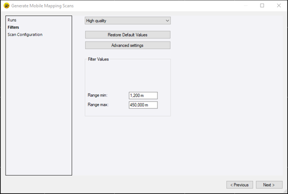
Choose between Default and High Quality.
Default contains the Isolated Points filter, set to On.
High Quality contains the Fog, and Sun filters for an MX50, and the Fog, Sun and Reflective Panels filters for an MX60, all set to On. On foggy days, a thick tunnel of very dark points at short distances around the trajectory of the vehicle may appear. The Fog option lets you filter these foggy parasites. On sunny days, a burst of points from the laser scanner toward a single direction in the sky may appear. The Sun option lets you filter these sunny parasites. The Reflective Panels option removes the noise before and after a target.
If required, click the Advanced Settings button.
Define either the minimum distance (Range Min.) or the maximum distance (Range Max.) to filter.
If required, click Restore Default Values:
Default: Isolated Points Off, Range Min. 0.50 meters and Range Max. 80 meters (for an MX50) or 150 meters (for an MX60).
High Quality: Fog On, Sun On, Reflective Panels filter On (only for an MX60), Range Min. 0.50 meters and Range Max. 80 meters or 150 meters (for an MX60). - Click Next. The last step is to compute the XYZ coordinates of the point cloud by converting the TMX format files to the RWCX format files. TBC uses the navigation and trajectory information file, i.e., the SBET or NAV file that has been set when importing the mission database file (*.mxdb) into the VCE project.
MX9 and MX90: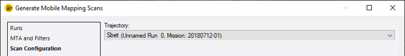
MX50 and MX60: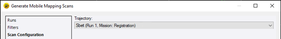
If you want to use a SBET file (or NAV file) other than the one set during the import, you can do this before extracting the mobile mapping scans from the raw data files. You have to first display the properties of the mission: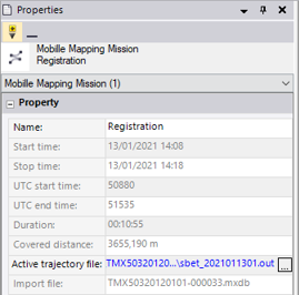
And click
 to open the Select Trajectory dialog from which you can choose another SBET file (or NAV file).
 - If required, colorize the laser point cloud that will be extracted with the RGB color values found in the video clip(s), i.e. the color information in the PGR format files. Check the Colorize Points With Panoramic View option. All the options in the Mask pane become enabled.
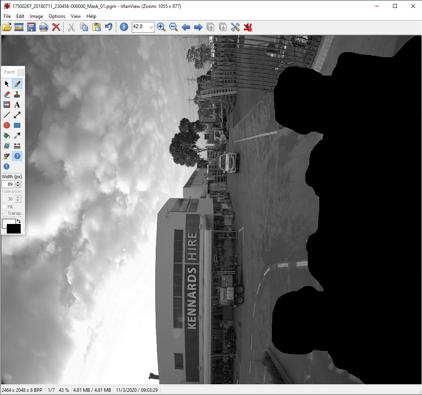
The principle of point cloud colorization is to create a Mask, on which any undesirable areas, objects and obstructions visible on the all images will be covered so that the color information found on them will be not used for the colorization.
In case there is no Mask available in the current project, the user needs to create one. The project has to be saved first in the TBC’ VCE format (if not already done). The Mask file will be saved then under the VCE project folder. If the project has not been saved, TBC will not find the path to a folder where the mask file will be put and will display an error message.
MX9 and MX90: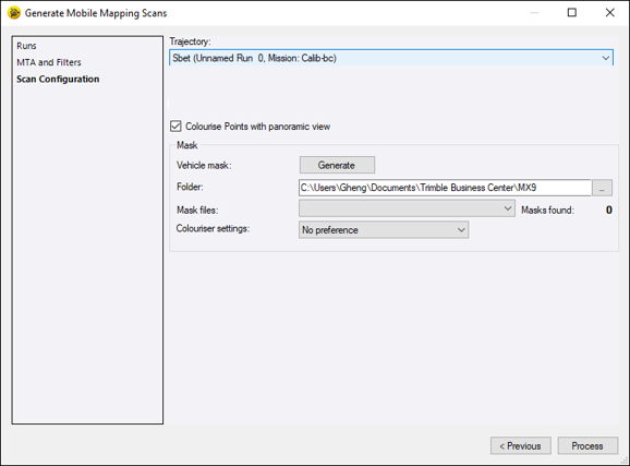
MX50 and MX60: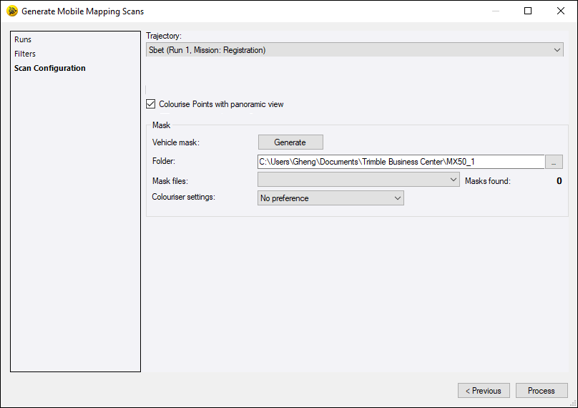
Note: You can use a mask coming from another project created using the same capture system settings by copying the masked images into the appropriate project folder. However, the capture system settings must be exactly the same.
- Click Generate.
Six Portable Grey Map image (PGM) files are created, one for each camera of the 360° camera. All are saved under theVCE project folder (if the project has been previously saved).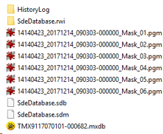
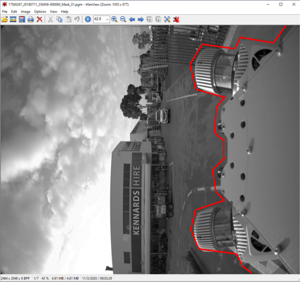
- Using a third party image editing software such as Irfanview, or GIMP, open a PGM format file and then color over the problem area (area surrounded in red in the picture below) using a fill color with 0,0 and 0 as RGB values.
Note: Do not rotate the PGM format files clockwise when coloring the unwanted area. Doing so may compromise the result of the colorization.
MX9 and MX90:
MX50 and MX60: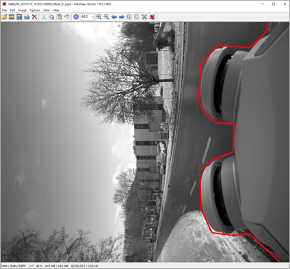
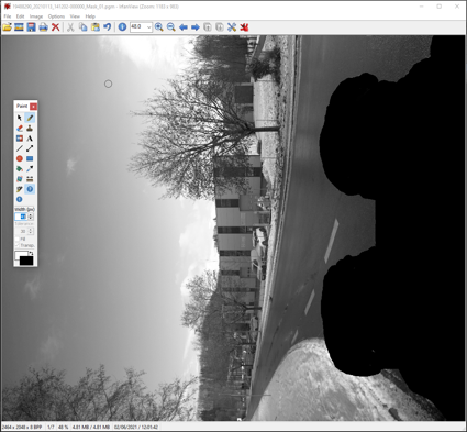
- Save the image using the same file name and location, overwriting the original PGM image file.
- Repeat the steps from 8 to 9 for the rest of the PGM image files.
- Drop-down the Colorizer Settings pull-down arrow.
- Select the direction from which to colorize:
No Preference uses no preference.
Prefer Backward Looking Sensors uses the sensors that are backward facing.
Prefer Forward Looking Sensors uses the sensors that are forward facing. - Click Process.
Note: To be able to process the RXP laser format files, you need to save your VCE project first. If not, the Save As dialog opens and prompts you to save it.
The Process View displays. You can follow the status of the extraction or stop the extraction by pressing the Cancel button.
At the end of the conversion, a dialog opens and lists the name of the current mission, the name of the processed run with/without the MTA option applied and/or the Colorization option applied.
MX9 and MX90: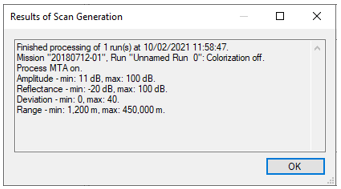
MX50: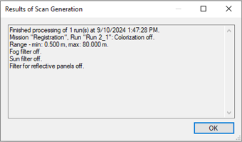
MX60: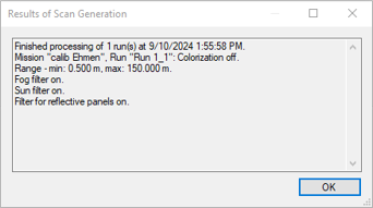
In the Project Explorer pane:
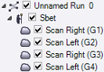
- A Point Cloud Region that includes all of the scan points is automatically created and displayed as the Default point cloud region node (1).
- Two Scan nodes (2) are created and nested beneath the imported trajectory of each selected run.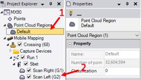
- A set of Stations is created and nested beneath the Scans node, with a Scan node inside.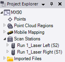
Note: In case of a single scanner configuration, only left or right station nodes and scan nodes are created.
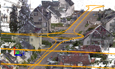
The extracted mobile mapping scans are displayed in the Plan View:
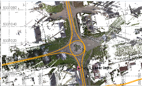
And in the 3D View:
Notes:
- The current VCE project will be saved automatically after the computation of the scan data.
- In case TBC closes unexpectedly, it is possible to recover already processed scans and see point clouds in the Plan View by tapping the “ComputeProject” command in the Command pane.
- The Scan nodes (beneath the imported trajectory of each selected run) are checked and the extracted scans are shown in the Plan View (or 3D View) only if the Show Scans After Generation option in the Mobile Mapping Options has been selected.You can use the Toggle Visibility command to display (or hide) the extracted scans in the Plan View (or 3D View).
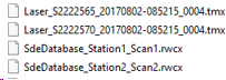
At the same time a set of files (TMX and RWCX) are created under the SdeDatabase folder under theVCE project:
Note: You cannot run two scan computations at the same time. If done anyway, an error message pops up.
AFTER extracting the mobile mapping scans from the raw data files, you are still allowed to change the SBET file (or NAV file) to use in your project. The Active Trajectory File file in the Properties pane is STILL enabled.
All the mobile mapping scans extracted from the selected run, with the same imported trajectory are put under the Import Trajectory node.
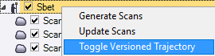
You can hide/display the imported trajectory of the selected run as well as the related mobile mapping scans and/or points (ground control points (GCP) and/targets) by selecting the Toggle Versioned Trajectory command from the pop-up menu or unchecking the related checkbox:
If the selected run has been already registered, you can select the resulting adjusted trajectory as trajectory input for generating the point cloud scan. If you have imported some trajectory files in your project (through the Properties window), you can select one to use for generating the point cloud scan.
MX9 and MX90: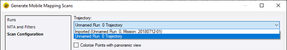
MX50 and MX60: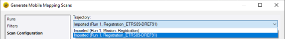
When you display the properties of a mobile mapping scan, you may see the filtering options and the trajectory file that have been used.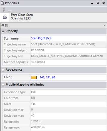
Note: Canceling the processing (extraction and colorization) of a large data set by clicking Cancel from the Process View tab may take time to react.
The time required to extract the mobile mapping scan data from a small section of a run is similar to the time for the entire run as the processing is done on the entire run.
