Understanding Vertical Designs

Fundamentals

Use ‘vertical design’ tools to rapidly create 3D models for roads, intersections, parking lots, site improvements, landscaping, and more from 2D linework. Vertical design functionality gives you a rule-based way to build such models using parametric instructions for elevations, cross-elevations, cross-slopes, long slopes, grades, breaklines, etc. to specify the geometric relationships between lines. This parametric approach means that you can easily adjust one rule or line’s geometry and have it modify the entire resulting surface. The rules have an order, so their dependencies build on each other.

Vertical designs are defined by:

Linear objects (CAD lines, linestrings, and alignments) which can be either 2D or 3D
Rules that parametrically define how selected lines geometrically relate to each other. To build the required model, use the various rule functions to instruct the process of converting lines into 3D structures.

The linework used can be either 2D or 3D CAD lines, linestrings, and alignments. Using the rules, the command will convert any 2D lines into 3D lines. To achieve a desired structure, use the different rule functions to instruct the process. The figure below shows an example of interactions between lines using a few rules.

The vertical design commands allow you to:

Create a vertical design - Use the Create Vertical Design command to build models from linework using a variety of rules (parametric instructions) for elevations, slopes, cross-slopes, grades, and other types of connections and transitions. This functionality provides a rule-based way to create 3D models for roads, intersections, parking lots, landscaping, and other site features. (See “Create a Vertical Design” in the TBC help.)
Edit a vertical design - After you have created a vertical design, use the Edit Vertical Design command to enter or modify parameters for a design. You can also use the Remove Line From a Vertical Design command to edit the design. When you are done making changes, use the Rebuild Vertical Design command to bring your model up-to-date with the updated design. (See “Edit a Vertical Design” in the TBC help.)
Add/remove lines from a vertical design - After you have created a vertical design, use the Remove Line from Vertical Design command to edit the design by taking a source or target line out of the computations. You can add new lines to a vertical design using the Lines tab in the Edit Vertical Design command. (See “Remove Lines from a Vertical Design” in the TBC help.)
Create a simple vertical design - Use the Create Global Vertical Design command to quickly and easily add one or more vertical design rules to a line or between two lines without needing to use the Create Vertical Design or Edit Vertical Design commands. The command pane prompts you for just the required parameters for the rule. See Create a Global Vertical Design.
Rebuild one or more vertical designs - When you are done making changes, use the Rebuild Vertical Design or Rebuild All Vertical Designs command to bring your model up-to-date with the updated design.
Note: You can rebuild either a single vertical design or all vertical designs at once. To rebuild one vertical design, right-click it in the Project Explorer, and select Rebuild Vertical Design. To rebuild all vertical designs, right-click the parent Vertical Designs node in the Project Explorer, and select Rebuild All Vertical Designs;all designs are rebuilt in the order shown in the explorer tree. Vertical designs are in alphabetical order there, so you can control the building order of the vertical designs with the naming. Building order may be significant because different vertical designs may contain the same objects, i.e., the target objects of the previous vertical design may be the source objects for the next vertical design.

This set of tools builds on the parametric intersection functions for modeling roundabouts, cul-de-sacs, ramps, and interchanges, and enables you to prepare data from 2D linework that defines the geometry of a target model. You can use vertical control rules to elevate lines that are then automatically added to a 3D vertical design model. You can also use vertical design tools to elevate lines to be added to an existing surface model built without the vertical design rules.

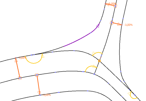
Figure 1: Linework and rules defining part of a model (a road intersection)

The parametric rules that you use are stored in TBC as children of their parent vertical design , much like other graphical objects (like the lines that use them). You can see the relationship between a design and its rules in the Project Explorer.

Rules for vertical designs are parametric: once you create a design, if you change any of the parameters (the lines, rules, or rule values), the design updates accordingly. You can have this update done automatically or only when you initiate it. This is what makes vertical design functionality so powerful. You design the structure of a model, how it is organized, and how to maintain it by adding or removing rules as needed. The structure of a design is visible because everything is graphically described.

Examples

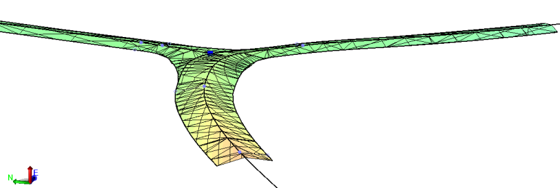
Figure 2: Model from Figure 1 seen in a 3D View

In this example, a few rules have been added to several lines for an intersection. To show the power of parametric design, a single cross-slope rule has been added between the lines at the forefront of the image, changing the slope from -3% to 3%. The result is shown in Figure 3 below.

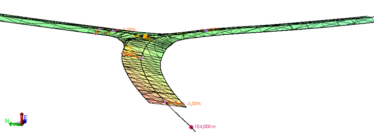
Figure 3: Change to model from the addition of a single cross-slope rule

With carefully defined rules, all lines in a vertical design can be connected correctly. Because there are many different situations to model, the ‘parametric vertical design’ includes a lot of ways in which lines can be connected. Currently, these methods will help you model most basic scenarios. Ultimately, parametric vertical design can be expanded with additional, more sophisticated methods that will make modeling even the most complex geometry easier.

Lines

The lines you select to create or edit a vertical design can be either:

2D (only horizontal geometry)
3D (horizontal and vertical geometry)

Locking/unlocking lines

Each line used in a vertical design has a property called Locked, which is set to either True or False. If a line is locked, it has write protection, which means that vertical rules (parameters) assigned to the line cannot be changed. If the Locked property for a line is set to False (off), the line will have only horizontal geometry when used to create a vertical design, even if it was originally a 3D line in your model, meaning that it is not affected by the vertical design rules. There are also Lock and Unlock rules you can apply to a section of a 3D line. For details, see Apply Lock and Unlock Rules.

Another fundamental principle for vertical designs in TBC is that all horizontal geometry used in a vertical design remains unchanged when creating the design. The Locked property can be found on the Lines tab when editing a vertical design.

Note: Locking/unlocking lines is different than making vertical design rules Active/Inactive, which means that a rule is not used in calculations.

Rules

There are three types of rules:

Point - This rule type applies a property (elevation, vertical point of intersection) to a specific point/station/distance along a line.
- Elevation rule - Apply this to a 2D line to make it 3D via one or more elevations. A surface is also created between vertices (as applicable) when you do this. For details, see Apply an Elevation Rule.
- Virtual break rule - Apply this to a 2D line to virtually split a line into sections without physically splitting it. For details, see Apply a Virtual Break Rule.
- Vertical PI rule - Apply this to a 2D line to make it 3D via one or more vertical points of intersection (VPIs). For details,Elevation line is a ‘point rule’ used to reduce the number of user-defined rules, such as Connector rules, required to copy an elevation from one line to another while elevating multiple lines from 2D to 3D. To apply it, simply specify a vertical radius and a start and end coordinate. All lines in between are computed with an elevation at the intersection point. see Apply a Vertical PI Rule.
- Crest/sag rule - Apply this to a 2D line to make it 3D by specifying an exact elevation of the sag or crest on the line (with the VPI Rule, it can be difficult to hit an exact line elevation because the property specifies a point of intersection (of tangents) and not the line itself). For details, see Apply a Crest/Sag Rule.
- Lock rule and Unlock rule - Apply this to prevent you from or allow you to edit a 3D line in order to change its vertical design. This function enables you to make changes in the vertical at specific areas of a line without losing verticals at other locations. For details, see Apply Lock and Unlock Rules.
- Elevation line rule - Apply this to to outer lines in a series to reduce the number of user-defined rules, such as Connector rules, required to copy an elevation from one line to another while elevating multiple lines from 2D to 3D. All lines in between are computed with an elevation at the intersection point. For details, see Apply an Elevation Line Rule.
  Note: Three types of rules can snap to many lines: Elevation rule, Elevate by dZ rule, and Elevate by Slope rule. If the rule is pointing to a location shared by many lines, all lines can be connected to the rule and its parameters. Such a common location can be the intersection of points, of lines, or their begin/end points.
  
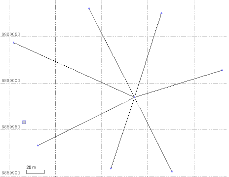
  This illustration shows a case in which many 2D lines meet at a common center point. If you apply a point rule at this center point (an Elevation rule for example), the rule (setting an elevation) will apply to all of the lines.
Arrow - This rule type applies a property (cross-slope, cross delta elevation, slope, delta elevation) between lines based on (and in the direction of) a starting point and an ending point.
- Cross-slope rule - Apply this from one line to another to create a sloped surface between them. If it elevates a target 2D line in the process, a surface is created between vertices on that line too. For details, see Apply a Cross-slope Rule.
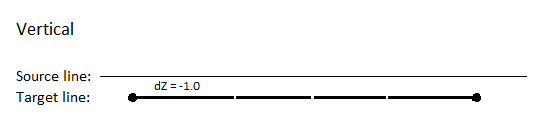
- Cross dZ rule - Apply this from a 3D line to another line to elevate the target line by a relative elevation change from the source line. For details, see Apply a Cross dZ Rule.
- Elevate by Slope rule - Apply this from a 3D line to another line to create a sloped surface between those points. Unlike cross-slope, it does not have to be connected to the source line (but it can). For details, see Apply an Elevate by Slope Rule.
- Elevate by dZ rule - Apply this from one location to another to elevate a target line by a relative elevation change from the source point. Unlike cross dZ, it does not have to be connected to a source line (but it can). For details, see Apply an Elevate by dZ Rule.
Other - This type encompasses the remaining unique rules that apply a property (grade, transition) to a single line or relationship (breakline, connector, tilt) between two lines.
- Grade rule - Apply this to compute a constant slope along a target line (the from and to points must be on the same line). For details, see Apply a Grade Rule.
- Breakline rule - Apply this to create extra 3D line work to improve the triangulation of surfaces. For details, see Apply a Breakline Rule.
- Transition rule - Apply this to compute a vertical connection between a starting point and an ending point along a target line. For details, see Apply a Transition Rule.
- Connector rule - Apply this to copy an elevation from one line to another. For details, see Apply a Connector Rule.
- Tilt rule - Apply this to compute a vertical alignment (VAL) dropped on a surface. The Tilt rule operates without interaction with other rules to handle unique tilt issues around shaping intersections, like roundabouts. For details, see Apply a Tilt Rule.

Chained Line Dependencies (the order of rules)

Each vertical design begins with a ‘source line’ and ends with a ‘target line’. Zero or more other lines may be included in the computations done between the source and target lines. Rules are added from line-to-line in this ‘chain’, and each rule is based on the vertical geometry of the line before it in this chain. The order of rules applied between each line, forms dependencies in the chain and a parametric relationship between all of the lines involved.

Both 2D and 3D lines can be source lines for their target lines in this ‘computational loop’. If a line is computed correctly, it is added to the list of subsequent lines and used in further computations. Therefore, the order of the rules applied in a vertical design has a critical effect on how accurately the resulting model is formed.

Example

This simple example shows how important rule order is in getting a successful result. Two 2D lines were selected for the design. These rules were applied:

Cross-slope - Defines a 3% slope from the source line to the target line.
Elevation - Sets the elevation of the source line to 10.

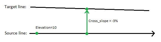
Figure: Plan view of an arrow rule being applied from a source line to a target line

If you apply the rules in this order:

Cross-slope order=1
Elevation order=2
the computation will fail because the source line is 2D when the cross-slope rule is executed; the target line will fail. When the Elevation rule is executed, the source line is computed correctly, but it unfortunately cannot not participate in computing the target line.

If you apply the rules in the opposite order:

Elevation order=1
Cross-slope order=2
the source line will first be computed using the Elevation rule, so it becomes a 3D line. When the cross-slope rule is executed, the source line can successfully compute the target line.
Note: In more complex situations, with many rules lined up, it is even more challenging to keep the order right, butthe basic principles are the same: the order of the rules is critically important.

Sectioning target lines

When a source line and a target line are connected by either a Cross-slope rule or Cross dZ rule, it is not necessary that the source line span the entire length of the target line. The lines can be non-coincident with each other as shown below in these four different, yet common, situations.

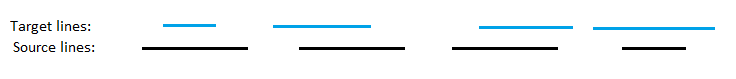
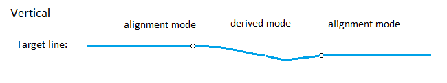
In each case, the target line is computed wherever it is located along the source line. If a section of the target line falls outside of the source line, the target line is ‘spilt’ into sections. To section a target line, it has to be open (not a closed line). Sectioning can happen (as shown above) both at the beginning and end of the target line, or at just one end. As shown below, the section that coincides with the source line has a derived vertical (derived mode). The rest has an ‘alignment’ vertical (alignment mode).

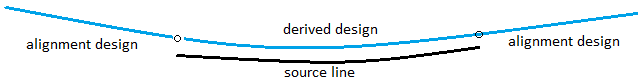
If no rules are defined for the alignment mode section, the elevation at the end of the derived mode section edge is extrapolated along the alignment section.

Of course, all types of vertical design rules can be applied along the alignment mode sections if needed.

Connecting Rules to Lines

There are two methods you can use to connect a rule to a line:

Search distance - This method looks for the nearest line within a radial distance from the point you pick when applying one of these point or other rules:
- Elevation
- VPI
- Connector
- Grade
- Transition
- Tilt
Hit length - This method looks for the nearest line by extension distance the vector created by two points you pick when applying one of these arrow rules:
- Cross-slope
- Cross dZ
- Elevate by slope
- Elevate by dZ
- Breakline

Using Search distance to connect a rule to a line

The figure below shows a situation in which a point is snapping to the nearest line using the Search distance method. If the perpendicular distance from the selected point to the line is is less than the specified Search distance, the connection is made. If many lines are within the Search distance, the nearest of them is selected. If no line is within the Search distance, no connection is made between the rule and the line.

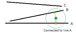
Figure: Point snapping to nearest line (line A) using the Search distance method

Both line A and line B fall within the search distance, but line A is selected because it is nearer to the point. Line C is ignored as too far away.

Using Hit length to connect a rule to a line

A ‘to’ and ‘from’ point must be specified to connect a rule to a line using the Hit length method. The figure below shows a situation in which a rule successfully connects a source line to a target line.

When searching forward for a target line, Line A and Line B are within the Hit length, which makes them candidates, while line C is too far away. Line A is nearer than line B, which makes Line A the target line.
When searching backwards for a source line, only Line D is within the Hit length, which makes it the only candidate and therefore the source line.

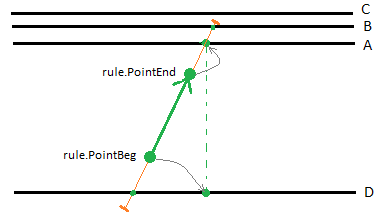
Figure: Snapping points to source and target lines

Note: The Hit length connects both the ‘from’ point to the source line and the ‘to’ point to the target line. The nearest line to the point within the tolerance is selected.

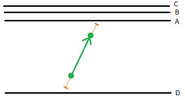
Figure: Snapping failed

If no lines are closer than the Hit length, the rule remains unconnected. To be connected correctly, both a source and a target line have to be found.

Adjusting rule geometry

All ‘arrow’ rules are defined by a start and an end point. Normally, these points are shown in graphic views to represent the original location of the rule. To get a correct graphical representation of the rule, points are computed at the ends of a perpendicular connection between the target and source lines.

For some rules, such as Cross-slope and Cross dZ, the to and from points are adjusted to be perpendicular to the source line. The figure above shows how the rule’s start point is adjusted to be perpendicular to its source line.

Tangential breaks on source lines

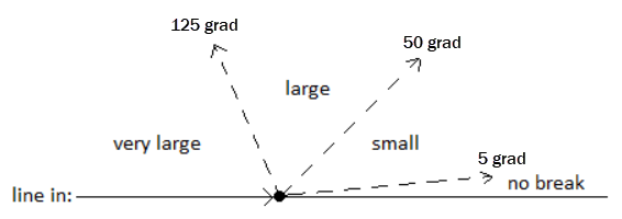
In this context, a tangential ‘break’ is a change of direction at a deflection point on a line; the direction to the break point is different than the direction from that point. The break is simply in relation to the horizontal alignment. The degree of angle of a tangential break on a source line affects the location of an arrow rule’s 'to' point on the target line. Breaks are measured in the unit called “grad”, which is also known as “gon”.

In other words, if tangential breaks occur on a source line that is used to compute derived geometry on a target line, the derived part of the target line is formed based on the break angle. Breaks are divided into following levels;

Note: You can set your horizontal angle units to grad in Project Settings > Units > Angle > Display > Grad.

No break (less than 5 grad)
Small break (from 5 to less than 50 grad)
Large break (from 50 to 125 grad)
Very large breaks (larger than 125 grad)

Since derived geometry is computed by offsetting from the source line, different break angles are computed differently to achieve smooth geometry.

Handling small breaks

In the example below, two target lines are passing the break point of the source line (one inside and one outside). Because the break angle is 5-50 grad, the small break method is used, but it affects the target lines differently:

The inside line has an overlap in the area affected by the break.
The outside line has a gap in the area affected by the break.

Handling the break this way is fine as long as the angle does not increase too much. When the break grows, the length of gap/overlap grows, and when break angle is 100 grad, it is infinite. Therefore, the small break is limited to 50 grad or less, If it is larger, it is a very large break and need another approach.

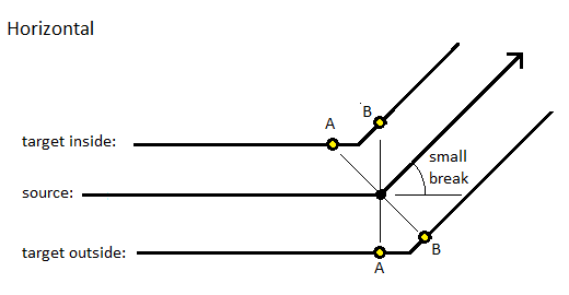
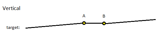
To find points A and B on the target lines, a perpendicular offset is computed a little before and a little after the break point on the source line. If the angle is very small, near the lower limit, the length of the overlap/gap on target line is very short.

Handling large breaks

If a tangential break’s angle is larger than 50 grad, a more specific method must be used. Inside and outside situations have to be handled separately.

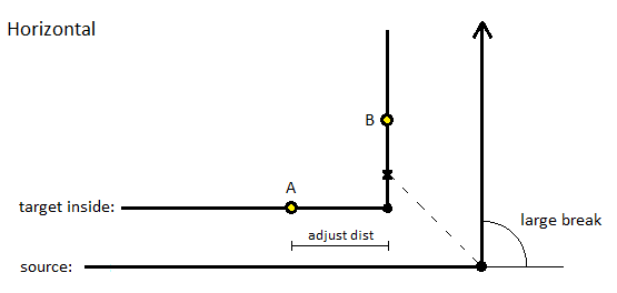
When the target line is inside of a source line with a large break, this process is applied:

The intersection point (x above) is computed by dividing the inside angle in 2, thereby making the intersection point a middle point.
If the target line has a break point near this middle/intersection point (adjust distance = 5.0 meter), the intersection point is moved to this break point (as shown above). If there is no break point on the target line, the intersection point remains at the middle point.
Points A and B are found by moving from the intersection point by the adjustment distance in both directions.
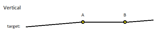
Depending on the derived geometry, points A and B might have different elevations (if the source line is elevated in this area). A straight line is drawn between A and B, as shown below. Notice that the elevation can change from A to B.

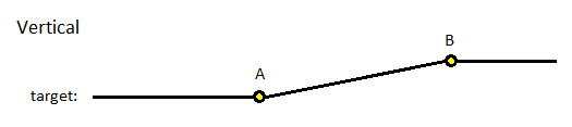
When the target line is outside of a source line with a large break, this process is applied:

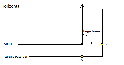
A perpendicular line is computed to the target line from the break point. Because of the break, there are two points: A and B. This outside case creates a gap. The elevations of A and B are not necessarily equal; they may vary based on the local offset distance, which not may be equal.

Handling very large breaks

If the break angle is more than 125 grad, the break is defined as very large. Parametric vertical design in TBC does not support this case.

If there are no breaks

The different states of tangential breaks are limited by parameters as noted previously. If a break is less than 5 grad, it is not handled as a tangential break; it is simply ignored. Because the break value is so small, it has minimal influence on vertical geometry: the overlap/gap area is close to zero. Only when the offset distance is very large can the overlap/gap length have any influence.

Applying a rule to a Cul-de-sac alignment

Alignments that end in cul-de-sacs can be designed in many ways. The figure below shows the ways in which a cul-de-sac alignment can be formed with a self-intersecting source line:

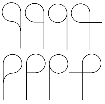
The shapes are (from left to right):

Tangential backward method (left/right)
Perpendicular method (left/right)
Tangential forward method (left/right)
Intersect method (left/right)

What is common to all of these examples is that the end of the line attaches to itself in one way or another. The source line can attach to itself tangential, perpendicular, or intersecting, and turn to the left or right (in the direction it is traveling or back on itself). At this time, only the tangential backward formation of a cul-de-sac is supported when adding an arrow rule.

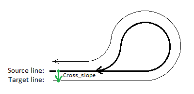
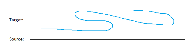
Figure: Plan view of a cul-de-sac source line inside a target line

In the figure above, the source line on the inside is 3D and the target line outside is 2D. If you need, for example, to add a cross-slope from the start to the end of the target line (even though the source line ends far up the road), you simply have to apply a single Cross-slope rule at the beginning of the source line.

Note: In some cases, the target line could be oriented in the opposite direction in relation to the source line (also called ‘backward direction’).

Handling target lines that change directions

Sometimes, a target line may deviate in direction (including in the opposite direction) from a source line. In some features, such as parking lots and trenches, this is common.

Therefore, the parametric vertical design is designed to compute derived geometry in cases where the target line changes direction in relation to the source line, especially where a section is perpendicular to the source line. The methods for handling these situations include:

Forward computation
Backward computation
Perpendicular computation.

If the target line is stationed in the same direction as the source line, the Forward computation is used. Here are some examples:

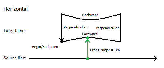
Case 1: Using Cross-slope to compute changing directions

In this case, a rectangular target line includes horizontal geometry that runs parallel and then perpendicular to the source line. The target geometry starts at the black dot and travels counter-clockwise (as shown by the arrow) from the start point to the end point (at the same location).

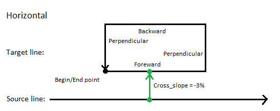
The 3D source line has a vertical alignment. The 2D target line will become 3D when the -3% Cross-slope rule is applied between source and target; only one cross-slope needs to be defined to compute the vertical. If desired, additional rules can be applied. The figure below shows in profile what comes out of this computation.

Note: The figure above is a schematic representation showing the underlying principle of the method.

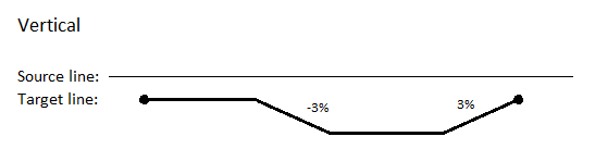
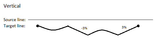
Notice that the first section (the forward) is computed with a constant horizontal offset distance, which makes the vertical constant also, since the slope is unchanged. The second section (the perpendicular out) adjusts the slope based on the negative cross-slope value. The third section (the backward) travels in the opposite direction of the source line.

It is not easy to see in the figure, but the target line is: reversed, then computed referring to the source line, and at last reversed back to the original direction. Finally, the fourth section (the perpendicular in) will also adapt slope value at current station at source line. Notice that the value will have opposite sign to Cross-slope value since it is opposite direction to the Cross-slope. Back again, the end point elevation is equal to the beginning point elevation.

Case 2: Using Cross dZ to compute changing directions

This case is similar to the previous one, with one difference: it uses a Cross dZ rule to define the elevation of the rectangle.

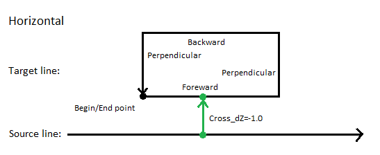
The entire target line is computed at the same elevation (as shown below).

This is the fundamental difference between this case and the previous one, where Slope-linearity was used to achieve vertical geometry. The input is similar, but the basic relationship between the source and the target has changed because of the difference between “source-linearity” and “offset-linearity”.

Case 3: Replacing Forward and Backward sections with arcs

In this case, the Forward and Backward sections have been replaced with arcs to show how changing offset distances in the horizontal have an effect on the vertical (as shown below)..

When horizontal offsets are changing, input to the vertical computation has to handle the change.

Because of slope-linearity, the vertical offset will vary as the horizontal distances change. Notice how this results in the variation of vertical geometry at given sections. If horizontal offsets increase, the vertical offset will increase (Forward) and opposite (Backward) by the formula:

dZ = slope * offset

where offset is the horizontal distance from the source line to the actual location on the target.

Derived combinations

The most common way of computing derived geometry is by having an open source line (not a closed shape) and a corresponding open target line that are generally parallel to each other.

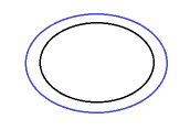
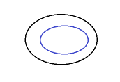
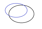
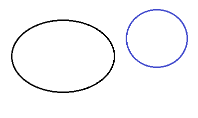
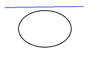
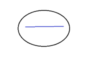
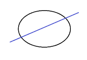
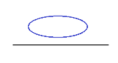
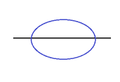
Twelve different, basic configurations are currently considered when computing vertical designs. Some of these configurations are supported, some are not supported, and the remainder have no solutions. In the graphics, the source line is black and the target line is blue.


Graphic	Status	Comment
	Supported	A closed target line is outside of a closed source line.
	Supported	A closed target line is inside of a closed source line.
	No possible solution	A closed target line intersects a closed source line.
	No possible solution	A closed target line has no intersection with a closed source line.
	Not supported	An open target line is outside of a closed source line.
	No possible solution	An open target line is inside of a closed source line.
	No possible solution	An open target line intersects a closed source line.
	Supported	A closed target line is outside of an open source line.
	Not supported	A closed target line intersects an open source line.

	Supported	An open target line is parallel to an open source line.
	Not supported	An open target line intersects an open source line.
	No possible solution	An open target line cannot possibly connect to an open source line.

Each of these configurations show which different geometric combinations are possible (among others). The parametric vertical design examples above are also represented to generate an appropriate status code and message for each case.